Overscoping and eval

In my previous post I used the lm function for an example of scope rules, but I left a few details out. I didn’t want to muddy the example with too many details, so I chose to lie a little.

The drawing I used to explain the example was this:

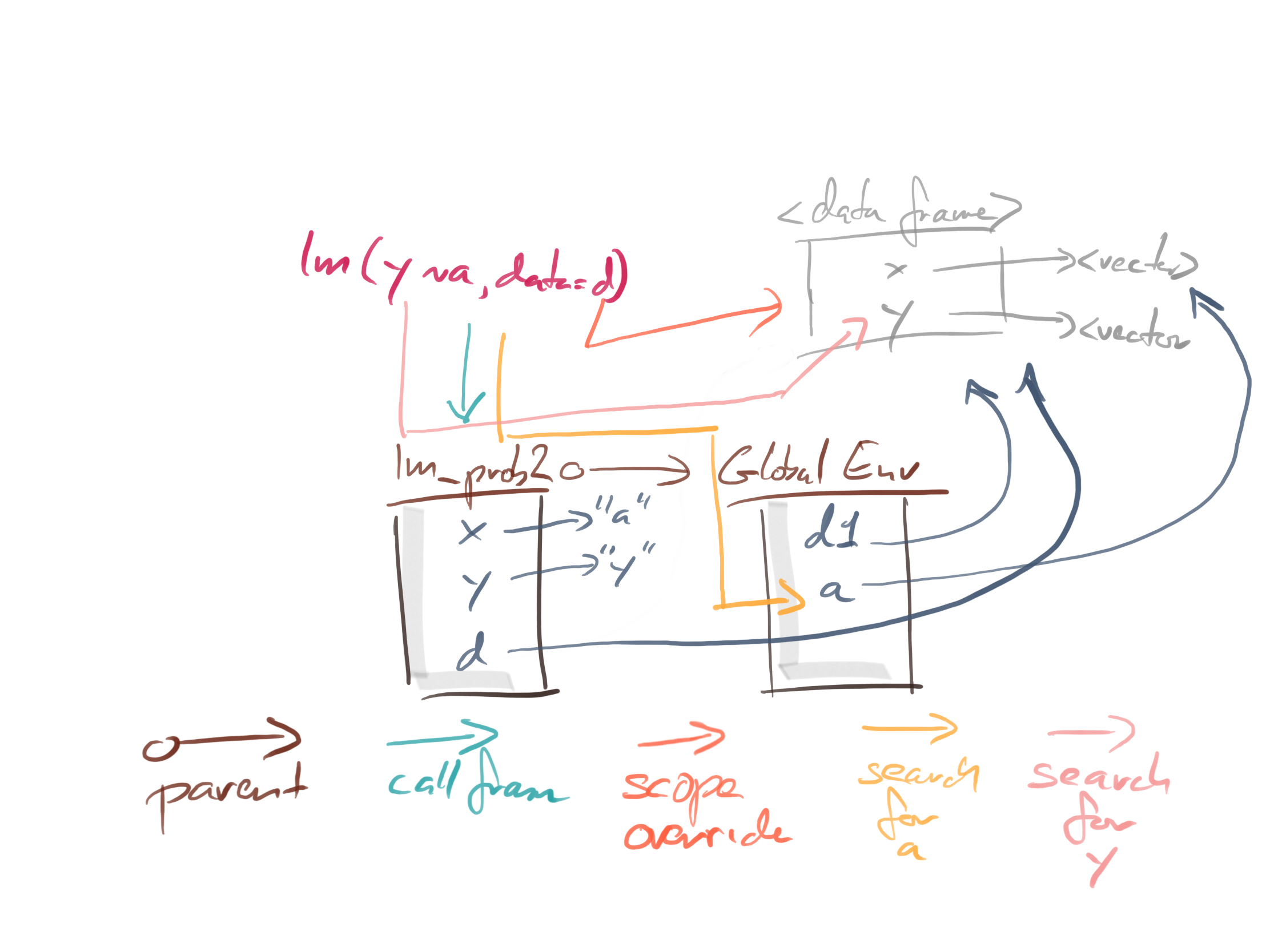
I explained how the scope is implemented using environments that are chained through parent pointers, and how a function has an environment associated with it. This environment is the environment where you define the function.

When you call a function, it gets its own instance environment (for historical reasons more than anything else we call this the call frame, but it is really just a new environment). The parent of that frame is the environment associated with the function.

So, we have two environments in play here, the environment of the instance and the environment where the function was defined. The parent of the former is the latter.

If you define a function nested inside another, then the environment associated with the nested function is the environment of the function call of the outer function. So, if you call the inner function, we have three environments in place: the one where the outer function was defined, the environment created when the outer function was called, and the environment of the inner function call.

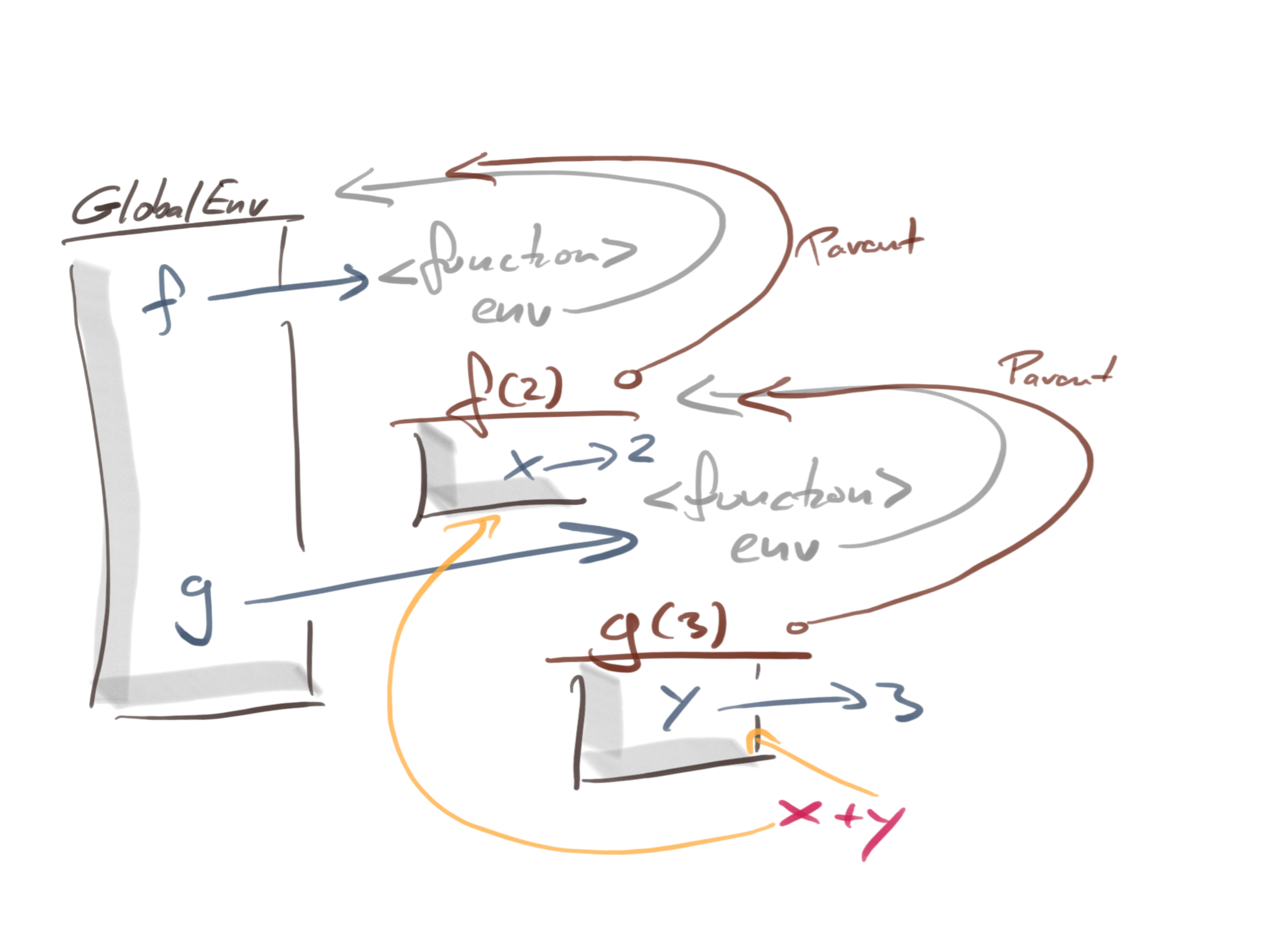
Consider this:

f <- function(x) function(y) x + y
g <- f(2)
g(3)

## [1] 5

The global environment will contain f and g. They are both variables in the global scope, and they are both functions, but the environment associated with them are different. Because f was defined in the global scope, that is the environment associated with. On the other hand, g was defined inside a call to f. We didn’t name it there, but what we name functions has nothing to do with where they are defined. The g function was defined inside the call to f.

In the call to f, we created an environment for the call, and we put the parameter x into this. The parent of this environment is the one associated with f, which is the global environment.

The environment associated with g is the one we created with the call to f, where we created the inner function. So, when we call g, we create an environment for the call, we set its parent to the one associated with g—the one we created when we called g. We put the parameter y into this environment, and it is in this environment we evaluate the body of g: x + y.

The setup is this, where I have illustrated where the g body finds variables x and y by searching through the environment chain, the y variable in the immediate environment and the x variable in its parent.

This is how lexical scope works.

Now, consider instead this code:

f <- function(x) x + y + z
g <- function(y) f(x)
h <- function(z) g(y)
x <- y <- z <- 1

What would happen if we called h(5) here?

h(5)

## [1] 3

The rules are the same as before, and the environments and how they are chained is this:

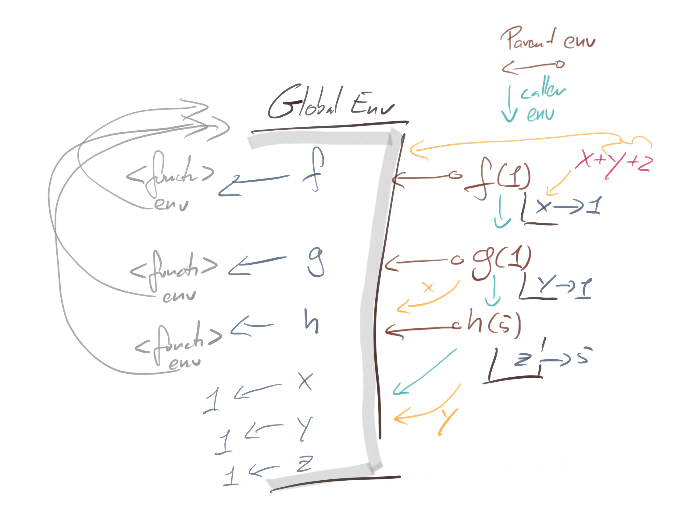
All three functions are associated with the global environment, so when we call them, that will be the parent of their call environments. This means that when we call h(5) we get an environment that maps z to 5, but we find the y we use in the call to g from the global environment, where it is 1. The call environment for g(y = 1) contains the mapping for y, but we find the x for the call f(x) in the global environment, so we call f(x = 1). That creates yet another call environment where we map x to one. When we evaluate x + y + z we find x in the call-environment, and we find y and z in its parent-environment—the global environment. That is why x + y + z evaluates to three.

I have shown the caller environments in blue-ish. For each function, it shows the environment where the function was called from. If R had so-called dynamic scope, the chain of blue environments is where it would look for the variables. But R implements lexical scope, so it follows the brown chains instead.

Non-standard evaluation

Now, we can explicitly tell R to use a different environment in which to evaluate an expression. We need to do two things: we have to replace expressions with quoted expressions and then evaluate them using the eval function with the alternative environment.

We have to use quoted expressions because otherwise, we will evaluate the expressions where we call eval and not inside it, in the environment we tell eval to do the evaluation.¹

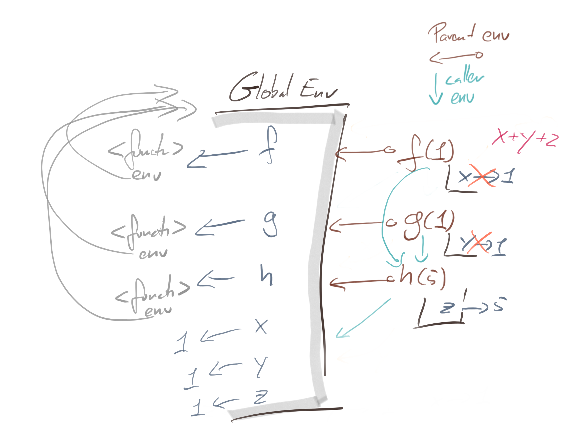
We can do something like this:

f <- function(x)
    eval(quote(x + y + z), rlang::caller_env())
g <- function(y)
    eval(quote(f(x)), rlang::caller_env())
h <- function(z) g(y)
h(5)

## [1] 7

This tells f to evaluate the expression x + y + z in the caller’s environment instead of its own. It tells g to evaluate the expression f(x) in its caller’s environment. Finally, we tell h just to evaluate g(y).

The chains of parents in this new setup is the same. Those are fixed once we have defined the functions.

You might also expect that the chains of caller-environments are the same, but that is not really true. The h function is still called from the global environment, and the g function is still called from h, so this doesn’t change. But inside the g call, we ask eval to pretend it is in the caller’s frame when it evaluates f(x), so the caller to f is h(5)’s environment.

To explicitly see the environments in place, we can out some output to the functions:

f <- function(x) {
    print("f's caller env:")
    print(rlang::caller_env())
    print("f's environment:")
    print(environment())
    eval(quote(x + y + z), rlang::caller_env())
}
g <- function(y) {
    print("g's caller env:")
    print(rlang::caller_env())
    print("g's environment:")
    print(environment())
    eval(quote(f(x)), rlang::caller_env())
}
h <- function(z) {
    print("h's caller env:")
    print(rlang::caller_env())
    print("h's environment:")
    print(environment())
    g(y)
}

When we call f from the global environment it has its own evaluation environment and the global environment as its caller’s environment:

f(x)

## [1] "f's caller env:"
## <environment: R_GlobalEnv>
## [1] "f's environment:"
## <environment: 0x7fbe64329698>

## [1] 3

The same when we call g, but when we ask eval to evaluate f(x) in g(y)’s caller environment we are asking it to evaluate f(x) in the global environment:

g(y)

## [1] "g's caller env:"
## <environment: R_GlobalEnv>
## [1] "g's environment:"
## <environment: 0x7fbe6540f3e0>
## [1] "f's caller env:"
## <environment: R_GlobalEnv>
## [1] "f's environment:"
## <environment: 0x7fbe65415d98>

## [1] 3

When we call h(5) we call it from the global environment, but we evaluate the g(y) call in h(5)’s evaluation environment:

h(5)

## [1] "h's caller env:"
## <environment: R_GlobalEnv>
## [1] "h's environment:"
## <environment: 0x7fbe65b33120>
## [1] "g's caller env:"
## <environment: 0x7fbe65b33120>
## [1] "g's environment:"
## <environment: 0x7fbe65b370e8>
## [1] "f's caller env:"
## <environment: 0x7fbe65b33120>
## [1] "f's environment:"
## <environment: 0x7fbe65e29168>

## [1] 7

So in this version, g will evaluate f(x) in h(5)’s environment and f will evaluate x + y + z in the same environment. When g evaluates x + y + z it finds z in the call-environment of h(5), and it finds x and y in the global environment (because this is the parent of h(5)’s environment). The environments of g(y) and f(x) are never in play here; we skip them entirely.

With me so far?

There is more to it than this. When g asks eval to evaluate quote(f(x)) in its caller’s environment, eval will also look for f there. Inside the scope of g(y), there is an f, and you can find it by going through its parent to the global environment. But that is not where eval looks for f. It looks for f starting in h(5)’s environment. It still finds f in the global environment, but if h had an inner function named f, that is where it would find it.

We haven’t implemented dynamic scope exactly here. We skip some local environments, but that is not what dynamic scope does. It looks through the chain of function calls to find its variables. We just skip some environments and avoid the local ones completely.

If you want dynamic scope you can set the parent of the local environments to the caller environment like this:

f <- function(x) {
    e <- environment() # the instance env.
    parent.env(e) <- rlang::caller_env()
    x + y + z
}
g <- function(y) {
    e <- environment() # the instance env.
    parent.env(e) <- rlang::caller_env()
    f(x)
}
k <- function(x, y, z) g(y)
k(1, 2, 3)

## [1] 6

When we call k(1, 2, 3) we define values for x, y, and z. We then call g(y), so we pass along the value of the local y. That value is stored in the variable y in the local environment of that call; it doesn’t matter here because both y variables refer to the same value, but we could change it in g, and the new value would be the one we see.

g <- function(y) {
    y <- -3 # change the binding of `y`
    e <- environment() # the instance env.
    parent.env(e) <- rlang::caller_env()
    f(x)
}
k(1, 2, 3)

## [1] 1

When we evaluate f(x) we have also changed the parent environment, so while we can find x in the local environment we search for y and z in the caller’s environment instead of our original parent’s.

Notice here that we no longer need to use eval for non-standard evaluation. When we change the parent of our environment, we can just evaluate expressions in the usual way.

If you want to combine lexical and dynamic scope, you are in a bit of trouble. Your environments only have one parent, so you have to either use the caller’s environment or the function’s environment.

You can mix the two by explicitly searching for variables in different environments, you can use the get function for this:

f <- function(x) {
    function(y) {
        z <- get("z", rlang::caller_env())
        x + y + z
    }
}
g <- f(1)
h <- f(2)
z <- 1
g(2) # 1(x) + 2(y) + 1(z)

## [1] 4

h(3) # 2(x) + 3(y) + 1(z)

## [1] 6

k <- function(z) g(2)
k(3) # 1(x) + 2(y) + 3(z)

## [1] 6

k(4) # 1(x) + 2(y) + 4(z)

## [1] 7

I wouldn’t recommend doing stuff like that, though. Dynamic scope is terrible enough as it is, and people expect lexical scope. R has enough functions with non-standard evaluation, but they work in a reasonably consistent way, so they do not cause much trouble.

If you get too inventive with environments, you are just setting yourself up for trouble.

Always code as if the guy who ends up maintaining your code will be a violent psychopath who knows where you live.

Over-scoping

This brings me back to the example where I started this post. The lm function. This function builds its model based on variables in its caller’s environment. If you give it a data frame, it will first look there for the variables, and if it does not find them, it will look in the caller’s scope.

This sounds a bit like it first looks in one place and then another, and it looks like it is chaining one environment’s parent to another.

It is actually both simpler and more complicated than that.

The simple stuff first: When you ask eval to evaluate a quoted expression, you can give it an environment to do it in. We have seen that in the examples above and in my previous post.

You can also give it a list to search in.

x <- 1 ; y <- 2
expr <- quote(x + y)
eval(expr)

## [1] 3

eval(expr, list(x = 4, y = 5))

## [1] 9

Data frames are just lists, so it is the same that happens if you give it a data frame.

d <- data.frame(x = 1:5, y = 1:5)
eval(expr, d)

## [1]  2  4  6  8 10

If we give eval a list that only has some of the variables, it will use those it finds there and get the others from the caller’s environment:

rm(x, y)
x <- 5
d <- data.frame(y = 1:5, z = 1:5)
eval(quote(x + y + z), d)

## [1]  7  9 11 13 15

We say that the list overrules the environment or that it over-scopes it.

This looks like it is using two environments, but it isn’t. A list is not an environment; it doesn’t have a parent environment either.

So what happens if we want eval to get some variables from a list and others from an environment that is not the immediate caller?

The function f below calls eval and that call will evaluate expr by first looking in the vars list and otherwise in the f call’s scope.

f <- function(x, y, expr, vars) eval(expr, vars)
expr <- quote(x + y + z)
f(1, 2, expr, list(z = 2))

## [1] 5

f(4, 5, expr, list(z = 5))

## [1] 14

If you want eval to look in the caller’s environment of a function, rather than the function call’s own environment, you give it a third argument:

g <- function(x, y, expr, vars) 
    eval(expr, vars, rlang::caller_env())
expr <- quote(x + y + z)
x <- y <- 5
g(1, 2, expr, list(z = 2))

## [1] 12

g(4, 5, expr, list(z = 5))

## [1] 15

x <- y <- 1
g(1, 2, expr, list(z = 2))

## [1] 4

g(4, 5, expr, list(z = 5))

## [1] 7

In this version, the variables in g’s call environment are ignored; eval looks in the global environment—the caller’s environment—not the local one.

The eval function takes two environment-like arguments, envir and enclos. These are the over-scoping environment and the enclosing environment. It first looks in envir for variables, and if that fails, it looks in enclos.

If envir is an environment, it never looks in enclos—that parameter is only used as a substitute for the parent environment when envir doesn’t have one, e.g. when it is a list or a data frame. The default value for envir is the caller’s environment, i.e. the environment where you call eval from. If you use a list here, the default for enclos is the caller’s environment.

So that is how eval deals with over scoping. It doesn’t combine dynamic and lexical scope, it just looks in a list before it searches an environment.

The reason that lm is slightly more complicated than this is that lm wants a formula as its first argument.

We can give it a formal and optionally a data frame to get some of the arguments:

x <- rnorm(5) ; y <- rnorm(5)
d <- data.frame(y = rnorm(5))
lm(y ~ x) # local x and y

## 
## Call:
## lm(formula = y ~ x)
## 
## Coefficients:
## (Intercept)            x  
##     -0.5451       0.6438

lm(y ~ x, data = d) # local x, data frame y

## 
## Call:
## lm(formula = y ~ x, data = d)
## 
## Coefficients:
## (Intercept)            x  
##     -0.2303       0.1089

We can also assign a formula to a variable and use that the same way:

f <- y ~ x
lm(f) # local x and y

## 
## Call:
## lm(formula = f)
## 
## Coefficients:
## (Intercept)            x  
##     -0.5451       0.6438

lm(f, data = d) # local x, data frame y

## 
## Call:
## lm(formula = f, data = d)
## 
## Coefficients:
## (Intercept)            x  
##     -0.2303       0.1089

However, formulae have their own environments, and these can work as closures. If you define a formula in a function, it will be associated with that function call’s environment.

environment(f) # f defined in the global env.

## <environment: R_GlobalEnv>

make_formula <- function(x) y ~ x
f2 <- make_formula(rnorm(5))
f3 <- make_formula(rnorm(5))
lm(f2) # f2 defined in a closure

## 
## Call:
## lm(formula = f2)
## 
## Coefficients:
## (Intercept)            x  
##     -0.3044       0.3571

lm(f3) # f3 defined in a closure

## 
## Call:
## lm(formula = f3)
## 
## Coefficients:
## (Intercept)            x  
##    -0.24855      0.05978

rm(x, y) # no global variables
ls(environment(f2)) # f2 still remember's an x

## [1] "x"

If we try to fit a linear model to f2 we get an error—there is no y variable anywhere.

lm(f2)

## Error in eval(predvars, data, env): object 'y' not found

We can still get it from the data frame, though

lm(f2, data = d)

## 
## Call:
## lm(formula = f2, data = d)
## 
## Coefficients:
## (Intercept)            x  
##     -0.2295       0.2595

Once you start passing formulae around in function calls, everything gets just a tad more complicated. Consider these two functions for building a linear model:

fit_model1 <- function(y) lm(x ~ y)
fit_model2 <- function(y) lm(f)

The first try to build a model from the formula x ~ y created inside the function call. It fails because we do not have any x variable in the function call’s environment or in its parent, the global environment.

fit_model1(rnorm(5))

## Error in eval(predvars, data, env): object 'x' not found

The second fails because we do not have the variable y in the formula’s environment—we have one in the function call’s environment, but the formula isn’t defined there, it was created in the earlier closure.

fit_model2(rnorm(5))

## Error in eval(predvars, data, env): object 'y' not found

The lm function first looks in the data frame you give it if any. If it doesn’t find the variables it needs there, it looks in the formula’s environment. It doesn’t look in the calling environment.

In the example that I started with it did look in the caller’s environment, but that was because we created the formula there.

As I said in the previous post: the rules for finding variables in environments are not that hard to understand. It is how they combine that makes things complicated. If you didn’t know that formulae have their own environments, then this could definitely be confusing. Now that you know they do, you can figure out why things don’t work as intended when that happens.

Formulae and function calls are not the only objects that carry environments with them. Function arguments do as well. But that will have to be another post. If you cannot wait, then have a look at Functional Programming in R, Metaprogramming in R, or Domain-Specific Languages in R.

If you liked what you read, and want more like it, consider supporting me at Patreon.